neutral theory on human disease variants

Human genomic disease variants: A neutral evolutionary explanation

gene function annotation - DAVID

DAVID-WS: a stateful web service to facilitategene/protein list analysis

Time scales of divergence andspeciation among natural populations and subspecies of Arabidopsis lyrata (Brassicaceae)

• Premise of the study: Plant populations that face new environments adaptand diverge simultaneously, and both processes leave footprints in theirgenetic diversity. Arabidopsis lyrata is an excellent species for studying these processes. Pairs of populations and subspecies of A. lyrata represent different stages of divergence. These populations are also known to be locally adapted and display various stages of emerging reproductive isolation.

• Methods: We used nucleotide diversity data from 19 loci to estimatedivergence times and levels of diversity among nine A. lyrata populations. Traditional distance-based methods and model-based clustering analysis were used to supplement pairwise coalescence-based analysis of divergence.

• Key results: Estimated divergence times varied from 130000 generations between North American and European subspecies to 39000 generations between central European and Scandinavian populations. In concordance with previous studies, the highest level of diversity was found in Central Europe and the lowest in North America and a diverged Russian Karhumäki population. Local adaptation among Northern and central European populations has emerged during the last 39000 generations. Populations that are reproductively isolated by prezygotic mechanisms have been separated for a longer time period of ∼70000 generations but still have shared nucleotide polymorphism.

• Conclusions: In A. lyrata, reproductively isolated populations started to diverge ∼70000 generations ago and more closely related, locally adapted populations have been separate lineages for ∼39000 generations. However, based on the posterior distribution of divergence times, the processes leading to reproductive isolation and local adaptation are likely to temporally coincide.

exploit - 开发、利用、剥削

Am I right to exploit him in this way?

但我用这种方法剥削他，合适吗？

strip somebody of sth. - 去除脱掉某人的什么东西

They strip him of his mystique.

phangorn - a really good tools for Phylogenetic analysis in R

1. http://bioinformatics.oxfordjournals.org/content/27/4/592.full

2. http://cran.r-project.org/web/packages/phangorn/

data(yeast)

tree <- NJ(dist.logDet(yeast))

fit <- pml(tree, yeast, k=4, inv= .2)

fit <- optim.pml(fit, optNni=TRUE, optGamma=TRUE, optInv=TRUE, model=“GTR”)

BS <- bootstrap.pml(fit, optNni=TRUE)

plotBS(fit$tree, BS, type = “phylogram”)

咀嚼、吞咽数据 - crunch data

crunch data

Tablet - next generation sequence assembly visualization

Please cite: Milne, I, Bayer, M, Cardle, L, Shaw, P, Stephen, G, Wright, F and Marshall, D. 2010. Tablet - next generation sequence assembly visualization. Bioinformatics 26(3), 401-402.

Tablet features:

• High-performance visualization and data navigation.
• Display of reads in both packed and stacked formats.
• File format support for ACE, AFG, MAQ, SOAP2, SAM, BAM, FASTA, FASTQ, and GFF3.
• Import GFF3 features and quickly find/highlight/display them.
• Search and locate reads by name or subsequence across entire data sets.
• Paired end visualization support (for SAM/BAM).
• Entire-contig overviews, showing data layout or coverage information.
• Simple install routine via auto-updating graphical installers.
• Support for Windows, Apple Mac OS X, Linux and Solaris, in 32 and 64-bit.

Reconstructing the origin and spread of horse domestication in the Eurasian steppe

http://www.pnas.org/content/109/21/8202.full

Model Fitting.

 

We fitted our model by using an approximate Bayesian computation framework, using the ABC-GLM algorithm implemented in the ABCtoolbox software (28). We used six summary statistics to describe our dataset: After assigning the sampled populations to three groups (west, central, and east, Fig. S2), we computed average within-population heterozygosities within each of the groups (three estimates) and average between-group heterozygosities (west vs. central, west vs. east, and central vs. east, three estimates).

We started by randomly sampling 55 million combinations of parameter values within the following ranges: t ∈ [500, 15,000] generations (corresponding to 6–180 kya), m ∈ [10⁻⁶, 10⁻³], cK ∈ [1, 10⁴], r ∈ [0.005, 1], K ∈ [4,000, 10⁵], K₀ ∈ [1, 10⁵], m_d ∈ [10⁻⁴, 0.5], K_d ∈ [500, 10⁴], c_dK_d ∈ [1, 10³], q ∈ [0, 1], and c_dK_d0∈ [1, 10³]. Whereas t and q were sampled according to the uniform distribution of their untransformed values, all other parameters were sampled from the uniform distribution of their log-transformed values. For each parameter value combination, we then generated our six summary statistics for each of the 12 scenarios, combining all possible origins for wild horses and domestication events in our model. In these calculations we took the mutation rate (μ) to be 1.5 × 10⁻⁴ per generation (the average of mutation rate estimates for two microsatellite markers, AHT4 and HTG10) (29). Because horse domestication occurred relatively recently, the only parameters that are considerably affected by the mutation rate are the time of the initial expansion of E. ferus in Eurasia (t) and the ancestral population size of E. ferus (K₀). For each scenario, we ran ABC-GLM on the accepted parameter combinations (on the basis of the 0.1 percentile of Euclidean distances between simulated and observed summary statistics) to estimate posterior distributions of the model parameters and the likelihood of the summary statistics as estimated from the genetics data (Table S2). We then used Bayes factors, given by the ratio of estimated likelihoods for each pair of scenarios, for model comparison. Because both Bayes factors and posterior distributions for a deme spacing of 100 km (Figs. 2 and 3) were in close agreement with those obtained for deme spacings of 50 km and 200 km, respectively (Figs. S3–S5), we refer to the former only in the main text.

EggLib - C++/Python library and program package for evolutionary genetics and genomics

1. De Mita S. and M. Siol. 2012. EggLib: processing, analysis andsimulation tools for population genetics and genomics. BMC Genet. 13:27.

2. http://egglib.sourceforge.net/index.html

3. the manual of PDF
http://ftp.jaist.ac.jp/pub/sourceforge/e/eg/egglib/current/egglib.pdf

4. an example

polymorphismBPP(dataType=1)
Computes diversity statistics using tools provided through the Bio++ libraries. Note that attempting to
call this method from an EggLib module compile without Bio++ support will result in a RuntimeError.
Arguments:
•dataType: 1 for DNA, 2 for RNA, 3 for protein sequences, 4 for standard codons, 5 for vertebrate
mitochondrial codons, 6 for invertebrate mitochondrial codons and 7 for echinoderm mitochondrial codons.
The method returns a dictionary containing the diversity statistics. Some keys will be computed only
in the presence of an outgroup, or if sequences were specified as coding or depending on the value of
other statistics (otherwise, they will be None).
The following statistics are always computed:
    •S: Number of polymorphic sites.
    •Sinf: Number of parsimony informative sites.
    •Ssin: Number of singleton sites.
    •eta: Minimal number of mutations.
    •thetaW: Theta estimator (Watterson Theor. Popul. Biol. 7:256-276, 1975).
    •T83: Theta estimator (Tajima Genetics 105:437-460, 1983)
    •He: Heterozygosity.
    •Ti: Number of transitions.
    •Tv: Number of transversions.
    •K: Number of haplotypes.
    •H: Haplotypic diversity.
    •rhoH: Hudson’s estimator of rho (Genet. Res. 50:245-250, 1987)

The following statistic is computed only if Tv > 0:
    •TiTv: Transition/transversion ratio.
The following statistic is computed only if S > 0:
    •D: Tajima statistic (Genetics 123:585-595, 1989).
The following statistics are computed only if eta > 0:
    •Deta: Tajima’s D computed with eta instead of S.
    •Dflstar: Fu and Li’s D* (without outgroup; Genetics 133:693-709).
    •Fstar: Fu and Li’s F* (without ougroup; Genetics 133:693-709).
The following statistic is computed only if an outgroup is found:
    •Sext: Mutations on external branches.

The following statistics are computed only if an outgroup is found and eta > 0:
      •Dfl: Fu and Li’s D (Genetics 133:693-709).
      •F: Fu and Li’s F (Genetics 133:693-709).
The following statistics are computed only if sequences are coding dataType = 4-7:
    •ncodon1mut: Number of codon sites with exactly one mutation.
    •NSsites: Average number of non-synonymous sites.
    •nstop: Number of codon sites with a stop codon.
    •nsyn: Number of codon sites with a synonymous change.
    •PiNS: Nucleotide diversity computed on non-synonymous sites.
    •PiS: Nucleotide diversity computed on synonymous sites.
    •SNS: Number of non-synonymous polymorphic sites.
    •SS: Number of synonymous polymorphic sites.
    •Ssites: Number of synonymous sites.
    •tWNS: Watterson’s theta computed on non-synonymous sites.
    •tWS: Watterson’s theta computed on synonymous sites

The following statistics are computed only if sequences are coding dataType = 4-7 and an outgroup is
found:
    •MK: McDonald-Kreitman test table (Nature 351:652-654, 1991).
    •NI: Neutrality index (Rand and Kann Mol. Biol. Evol. 13:735-748).
The returned dictionary also contains a nest dictionary options which feedbacks the values used
at function call. Changed in version 2.0.2: The following statistics are now computed only if S > 0:
D, Deta, Dflstar, Fstar, Dfl, F. Changed in version 2.1.0: The statistics not computed are now
exported and set to None.

Arlequin - could be run on Linux

1. Arlequin suite ver 3.5: a new series of programs to perform population genetics analyses under Linux and Windows
http://onlinelibrary.wiley.com/doi/10.1111/j.1755-0998.2010.02847.x/full

2. http://popgen.unibe.ch/software/arlequin35/Arl35Downloads.html

3.

Implemented methods

The analyses Arlequin can perform on the data fall into two main categories: intra-population and inter-population methods. In the first categorystatistical information is extracted independently from each population, whereas in the second category, samples are compared to each other.

Intra-population methods

Standard indices		Some diversity measures like the number of polymorphic sites, gene diversity
Molecular diversity		Calculates several diversity indices like nucleotide diversity, different estimators of the population parameter
Mismatch distribution		The distribution of the number of pairwise differences between haplotypes, from which parameters of a demographic or spatial population expansion can be estimated
Haplotype frequency estimation		Estimates the frequency of haplotypes present in the population by maximum likelihood methods
Gametic phase estimation		Estimates the most like gametic phase of multi-locus genotypes using a pseudo-Bayesian approach (ELB algorithm)
Linkage disequilibrium		Test of non-random association of alleles at different loci
Hardy-Weinberg equilibrium		Test of non-random association of alleles within diploid individuals
Tajima’s neutrality test		Test of the selective neutrality of a random sample of DNA sequences or RFLP haplotypes under the infinite site model
Fu's neutrality test		Test of the selective neutrality of a random sample of DNA sequences or RFLP haplotypes under the infinite site model
Ewens-Watterson neutrality test		Tests of selective neutrality based on Ewens sampling theory under the infinite alleles model
Chakraborty’s amalgamation test		A test of selective neutrality and population homogeneity. This test can be used when sample heterogeneity is suspected
Minimum Spanning Network (MSN)		Computes a Minimum Spanning Tree (MST) and Network (MSN) among haplotypes. This tree can also be computed for all the haplotypes found in different populations if activated under the AMOVA section

Inter-population methods

Search for shared haplotypes between populations		Comparison of population samples for their haplotypic content. All the results are then summarized in a table
AMOVA		Different hierarchical Analyses of Molecular Variance to evaluate the amount of population genetic structure
FST-Pairwise genetic distances		FST-based genetic distances for short divergence time
Pairwise moecular distances		Molecular distancess between populations based on the number of pairwise differencs between haplotypes
delta-mu square		Genetic distance betwene populations based on microsatellite data
Exact test of population differentiation		Test of non-random distribution of haplotypes into population samples under the hypothesis of panmixia
Assignment test of genotypes		Assignment of individual genotypes to particular populations according to estimated allele frequencies
Detection of loci under selection from F-statistics		Detection of loci under selection by the examination of the joint distribution of FST and heterozygosity under a hierarchical island model.

Mantel test

Correlations or partial correlations between a set of 2 or 3 matrices

SeqMaT: A sequence manipulation tool for phylogenetic analysis

http://www.ncbi.nlm.nih.gov/pmc/articles/PMC3044431/
http://glee.ist.unomaha.edu:8080/seqmat/downloads.jsp

Most bioinformatics tools require specialized input formats for sequence comparison and analysis. This is particularly true for molecular phylogeny programs, which accept only certain formats. In addition, it is often necessary to eliminate highly similar sequences among the input, especially when the dataset islarge. Moreover, most programs have restrictions upon the sequence name. Here we introduce SeqMaT, a Sequence Manipulation Tool. It has the following functions:

1. data format conversion,
2. sequence name coding and decoding,
3. redundant and highly similar sequence removal, and
4. data mining utilities. SeqMaT was developed using Java with two versions, web-based andstandalone. A standalone program is convenient to manipulate a large number of sequences, while the web version will guarantee wide availability of the tool for researchers and practitioners throughout the Internet.

Availability

The database is available for free at http://glee.ist.unomaha.edu/seqmat

Sequence analysis scripts

Sequence analysis perl scripts for fasta format

How can I count SNPs in my VCF files

http://www.biostars.org/post/show/49386/how-can-i-count-snps-in-my-vcf-files/

rm -f all.vcf
egrep -v "^#" SNP_chr1_EXOME.vcf |
awk -F ' ' ($1=="1" && int($2)>=11531680 && int($2)<=11631919)'  >> all.vcf

(...same for the other regions... )

cut -d ' ' -f1,2,4,5 < all.vcf |
sort -t ' ' -k1,1 -k2,2 -k3,3 -k4,4 |
uniq |
wc -l

how to automatically run a bash script when my qsub jobs are finished on a server

http://stackoverflow.com/questions/3886168/how-to-automatically-run-a-bash-script-when-my-qsub-jobs-are-finished-on-a-serve

two NGS tools

1. MolBioLib

MolBioLib is a compact efficient C++11 programming framework with accompanying set of tools enabling rapid developmentand deployment of next-generation sequencer data analysis programs. The library includes objects to aid in storage of relationaldata, traversal of delimited files, and manipulation of sequence files. Methods range from alignment writers to statisticalfunctions and string manipulations. Tools to manipulate TSV files, count aligned hits to features such as genes, coverage, andChIP-Seq are included.

2. GenomicTools
GenomicTools is a flexible computational platform for the analysis and manipulation of high-throughput sequencing datasuch as RNA-seq and ChIP-seq. GenomicTools implements a variety of mathematical operations between sets ofgenomic regions thereby enabling the prototyping of computational pipelines that can address a wide spectrum of tasksfrom preprocessing and quality control to meta-analyses. More specifically, the user can easily create average readprofiles across transcriptional start sites or enhancer sites, quickly prototype customized peak discovery methods forChIP-seq experiments, perform genome-wide statistical tests such as enrichment analyses, design controls viaappropriate randomization schemes, among other applications. In addition to enabling rapid prototyping, theGenomicTools platform is designed to analyze large-datasets in a single-pass fashion in order to minimize memory andintermediate file requirements. Finally, the GenomicTools platform supports the widely used BED format to facilitatevisualization as well as integration with existing platforms and pipelines such as Galaxy or BioConductor.

a special issue on Ecological Speciation

http://www.hindawi.com/journals/ijeco/si/213683/

关于 - pertain to

As GWAS applications have evolved so too have the community standards that pertain to them.

really nice map generated by R

http://dsparks.wordpress.com/2012/07/18/mapping-public-opinion-a-tutorial/

Septin-Mediated Plant Cell Invasion by the Rice Blast Fungus, Magnaporthe oryzae

http://www.sciencemag.org/content/336/6088/1590.full

To cause rice blast disease, the fungus Magnaporthe oryzae develops a pressurized dome-shaped cell called an appressorium, which physically ruptures the leaf cuticle to gain entry toplant tissue. Here, we report that a toroidal F-actin network assembles in the appressorium bymeans of four septin guanosine triphosphatases, which polymerize into a dynamic, hetero-oligomeric ring. Septins scaffold F-actin, via the ezrin-radixin-moesin protein Tea1, andphosphatidylinositide interactions at the appressorium plasma membrane. The septin ringassembles in a Cdc42- and Chm1-dependent manner and forms a diffusion barrier to localize theinverse-bin-amphiphysin-RVS–domain protein Rvs167 and the Wiskott-Aldrich syndrome proteinLas17 at the point of penetration. Septins thereby provide the cortical rigidity and membranecurvature necessary for protrusion of a rigid penetration peg to breach the leaf surface.

隐藏，潜伏 - lurk

Preventing a Disease Lurking in Her Genome

on role of an expansion of copy number of a chitin-binding domain in the amphibian pathogen B. dendrobatidis

Species-Specific Chitin-Binding Module 18 Expansion in the Amphibian Pathogen Batrachochytrium dendrobatidis

减弱坏的影响 - mitigate the effects

Two approaches to mitigating the eff ects of LD are to include markers that are separated from each other by a certain genetic distance, or to thin the markers according the observed sample correlation coeffi cients.

The Path from C3 to C4 Photosynthesis

"The Path from C3 to C4 Photosynthesis"

Peter Westhoff (Univ. Düsseldorf) recent publications include:

1. Regulation of the photorespiratory GLDPA gene in C(4) flaveria: an intricate interplay of transcriptional and posttranscriptional processes. Wiludda C, Schulze S, Gowik U, Engelmann S, Koczor M, Streubel M, Bauwe H, Westhoff P.

Plant Cell. 2012 Jan;24(1):137-51.


2. Evolution of C4 photosynthesis in the genus Flaveria: how many and which genes does it take to make C4? Gowik U, Bräutigam A, Weber KL, Weber AP, Westhoff P.

Plant Cell. 2011 Jun;23(6):2087-105.


3. The path from C3 to C4 photosynthesis. Gowik U, Westhoff P.

Plant Physiol. 2011 Jan;155(1):56-63.


4. An mRNA blueprint for C4 photosynthesis derived from comparative transcriptomics of closely related C3 and C4 species. Bräutigam A, Kajala K, Wullenweber J, Sommer M, Gagneul D, Weber KL, Carr KM, Gowik U, Mass J, Lercher MJ, Westhoff P, Hibberd JM, Weber AP.

Plant Physiol. 2011 Jan;155(1):142-56.

Recombination Rate Is Spatially Correlated with W→S DAF Skew across the Genome

Ongoing GC-Biased Evolution Is Widespread in the Human Genome and Enriched Near Recombination Hot Spots

Recombination Rate Is Spatially Correlated with W→S DAF Skew across the Genome

To further explore the relationship of W→S DAF skew and recombination, we correlated the W→S DAF skew in windows across the genome with the estimated recombination rate for each window for the YRI population from HapMap (The International Hapmap Consortium 2007). At a 40 kb window size, the raw Spearman correlation across the entire genome is 0.20 (P ≈ 0). When larger 1 Mb windows are considered, the correlation becomes much stronger (ρ = 0.53; P ≈ 0). Figure 5 illustrates this strong spatial correlation between bias and recombination rate across chromosome 2 (ρ= 0.43; P ≈ 0). The dramatic increase in correlation with increasing window size is consistent with models of the evolution of recombination hot spots in which there is a large amount of local variation between individuals and over time, but this variation is mainly contained within larger-scale regions with fairly constant recombination rates (Myers et al. 2005).

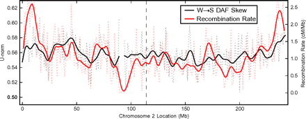
W→S fixation bias and recombination rate are significantlycorrelated across the genome. The W→S DAF skew (black) (asdescribed in fig. 2) and YRI population–based recombination rate (red) are significantly correlated (ρ = 0.62 smoothed and ρ = 0.43 unsmoothed; both P ≈ 0) across chromosome 2. Raw W→S DAF skew and recombination rate data in 1 Mb windows are plotted with dotted lines, and the data smoothed using a Hanning window of size 12 Mb are shown with solid lines. The dashed vertical line indicates the location of the fusion of two ancestral chromosomes on the human lineage.

Guidelines for Preparing Effective Presentations

https://honglangwang.wordpress.com/2012/07/16/guidelines-for-preparing-effective-presentations/

The following is from JSM:

Guidelines for Preparing Effective Presentations

These tips apply regardless of whether the time for the presentations isshort (less than 30 minutes) or long. Complaints about poorpresentations have been received for decades and continue to bereceived. The ASA has offered a short-course on presentation for manyyears, and routinely sends “tips” to speakers to promote effectivepresentations, but often go ignored. The tips and suggestions are hereto help you. Please put them to good use. An ad hoc committee(consisting of A. Lawrence Gould, Chair; Howard Kaplan; Peter ALachenbruch; and Katherine Monti) was formed at the April 1999 ENARbusiness meeting, to address this persistent and pervasive problem.Effective presentations make learning and technical advances morelikely. They also enhance the perception of the presenter in the eyes ofthe professional community. Boring, ineffective presentations are notpaid much attention and often are quickly forgotten, especially byplanners of future invited sessions.

Preparation

Content organization

• Make sure the audience walks away understanding the five things any listener to a presentation really cares about:
  a. What is the problem and why?
  b. What has been done about it?
  c. What is the presenter doing (or has done) about it?
  d. What additional value does the presenter’s approach provide?
  e. Where do we go from here?
• Carefully budget your time, especially for short (e.g., 15 minute)presentations.
• Allow time to describe the problem clearly enough for the audience to appreciate the value of your contribution. This usually will take more than 30 seconds.
• Leave enough time to present your own contribution clearly. This almost never will require all of the allotted time.
• Put your material in a context that the audience can relate to.It’s a good idea to aim your presentation to an audience ofcolleagues who are not familiar with your research area. Yourobjective is to communicate an appreciation of the importanceof your work, not just to lay the results out.
• Give references and a way to contact you so those interested in the theoretical details can follow up.

Preparing effective displays

Here are some suggestions that will make your displays more effective.

• Keep it simple. The fact that you can include all kinds of cute decorations, artistic effects, and logos does not mean that you should. Fancy designs or color shifts can make the important material hard to read. Less is more.
• Use at least a 24-point font so everyone in the room can readyour material. Unreadable material is worse than useless – itinspires a negative attitude by the audience to your work and,ultimately, to you. NEVER use a photocopy of a standard printedpage as a display – it is difficult to overstate how annoying thisis to an audience.
• Try to limit the material to eight lines per slide, and keep the number of words to a minimum. Summarize the main points – don’t include every detail of what you plan to say. Keep it simple.
• Limit the tables to four rows/columns for readability. Sacrificecontent for legibility – unreadable content is worse than useless.Many large tables can be displayed more effectively as a graphthan as a table.
• Don’t put a lot of curves on a graphical display – busy graphical displays are hard to read. Also, label your graphs clearly with BIG, READABLE TYPE.
• Use easily read fonts. Simple fonts like Sans Serif and Arial are easier to read than fancier ones like Times Roman or Monotype Corsiva. Don’t use italic fonts.
• Light letters (yellow or white) on a dark background (e.g., darkblue) often will be easier to read when the material is displayedon LCD projectors.
• Use equations sparingly if at all – audience members not working in the research area can find them difficult to follow as part of a rapidly delivered presentation. Avoid derivations and concentrate on presenting what your results mean. The audience will concede the proof and those who really are interested can follow up with you, which they’re more likely to do if they understand your results.
• Don’t fill up the slide – the peripheral material may not make itonto the display screen – especially the material on the bottomof a portrait-oriented transparency.
• Identify the journal when you give references: Smith, Bcs96 clues the reader that the article is in a 1996 issue of Biometrics, and is much more useful than just Smith 1996.
• Finally, and this is critical, always, always, always preview your presentation. You will look foolish if symbols and Greek letters that looked OK in a WORD document didn’t translate into anything readable in POWERPOINT – and it happens!

Timing your talk

Don’t deliver a 30-minute talk in 15 minutes. Nothing irritates anaudience more than a rushed presentation. Your objective is to engagethe audience and have them understand your message. Don’t floodthem with more than they can absorb. Think in terms of what it wouldtake if you were giving (or, better, listening to) the last paper in the lastcontributed paper session of the last day. This means:

• Present only as much material as can reasonably fit into the time period allotted. Generally that means 1 slide per minute, or less.
• Talk at a pace that everybody in the audience can understand. Speak slowly, clearly, and loudly, especially if your English is heavily accented
• PRACTICE, PRACTICE, PRACTICE. Ask a colleague to judge your presentation, delivery, clarity of language, and use of time.
• Balance the amount of material you present with a reasonable pace of presentation. If you feel rushed when you practice, then you have too much material. Budget your time to take a minute or two less than your maximum allotment. Again, less is more.

Loose ends

• PRACTICE, PRACTICE, PRACTICE the presentation, with care to content, delivery and use of time. (In case you missed this recommendation above)

The Presentation

• Put on the microphone and be sure that it works before you begin.
• Be sure everyone in the room can see your material. Make sure you do not block the screen. Move around if you must so that everyone has a chance to see everything.
• Never apologize for your displays. More to the point, makeapologies unnecessary by doing the material properly in the firstplace (see the recommendations above). Do not say, “I knowyou can’t see this, but…” The reaction of many people in theaudience will be “why bother showing it, then?” (Or, evenworse, “Why didn’t you take the trouble to make themlegible?”)
• Don’t apologize for incomplete results. Researchers understand that all research continues. Just present the results and let the audience judge. It is okay to say, “work is on-going”. Do not say, “I’m sorry that work is not done.” This invites the audience to tune out or wonder why you are talking at all.

When Finished

• Thank the audience for their attention
• Gather you materials and move off quickly to allow the nextpresenter to prepare
• Stay for the entire session

The following is from the post:

1. When giving an invited talk at a general TCS conference, do not assume that everyone in the audience isinterested in the technicalities of your subject. Focus onthe main message, tell the story of the ideas and whyyou think they are important. Give everyone somethingto take home.
2. Do not assume that you do not need to introduce thesetting for your work because someone else has done itbefore or on an earlier conference day. Not everyone willhave attended the talks where the background andmotivation were presented.
3. Do not run over time.
4. Never speak with your hands on your mouth, even if it feels good 
5. Do not let your voice drop to an inaudible level as your sentence progresses. Dare to speak slowly and loudly.
6. Ask yourself: How many slides do I really need for a 20-minute talk? Most of us will only use a few, and those should convey the message of the talk at a suitable level of abstraction.

The advice we give others is the advice we ourselves need.