guides on generating map plot with R

I collected these guides around the blog posts I found. Please go to the originals for details. And reference should go to the original authors.

1.  Japan Quake Map, with codes and video

library (ggplot2)

library (mapproj)

library (maps)

library (maptools)

# setting parameter about a map.

long <- c (120, 150)

lat <- c (25, 50)

# Reading data of earthquakes and map.

url <- "http://knowledgediscovery.jp/data/eq39.csv"

eq <- read.csv(url, as.is=T)

map <- data.frame(map(xlim = long, ylim = lat))

# creating image with ggplot.

p <- ggplot(eq, aes(long, lat))

p + geom_path(aes (x, y), map) +

geom_point(aes(size = Magnitude, colour = Magnitude), alpha = 1/2) + xlim(long) + ylim(lat)

Created by Pretty R at inside-R.org


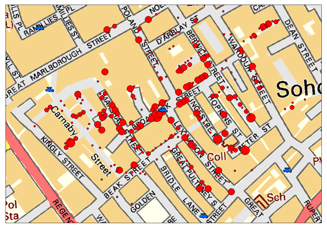
2. John Snow’s famous cholera analysis data in modern GIS formats, work with shape point format.

install.packages(“maptools”)

library(maptools)

deaths <- readShapePoints(“Cholera_Deaths”)

pumps <- readShapePoints(“Pumps”)

deaths # Prints out the deaths data – shows all of the attributes (count and ID in this case) plus the X and Y co-ords

# Create a simple (horrible) plot of the data

plot(deaths, col=’red’)

points(pumps, col=’blue’)

Created by Pretty R at inside-R.org



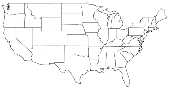
3. How to draw good looking maps in R, 

library(ggplot2)

library(maps)

#load us map data

all_states <- map_data("state")

#plot all states with ggplot

p <- ggplot()

p <- p + geom_polygon( data=all_states, aes(x=long, y=lat, group = group),colour="white", fill="grey10" )

p

Created by Pretty R at inside-R.org



4. Visualizing GIS data with Rand Open Street Map,
OpenStreetMap, and R package - RgoogleMaps

# (1) download the map

lat_c<-51.47393

lon_c<-7.22667

bb<-qbbox(lat = c(lat_c[1]+0.01, lat_c[1]-0.01), lon = c(lon_c[1]+0.03, lon_c[1]-0.03))



# download the corresponding Openstreetmap tile with the following line

OSM.map<-GetMap.OSM(lonR=bb$lonR, latR=bb$latR, scale = 20000, destfile=”bochum.png”)



# (2) Add some points to the graphic

lat <- c(51.47393, 51.479021)

lon <- c(7.22667, 7.222526)

val <- c(10, 100)



# As the R-package was mainly build for google-maps, the coordinates need to be adjusted by hand. 

# I made the following functions, that take the min and max value from the downloaded map.



lat_adj<-function(lat, map){(map$BBOX$ll[1]-lat)/(map$BBOX$ll[1]-map$BBOX$ur[1])}

lon_adj<-function(lon, map){(map$BBOX$ll[2]-lon)/(map$BBOX$ll[2]-map$BBOX$ur[2])



# (3) add some points to the map. If you want them to mean anything it may be handy to specify 

# an alpha-level and change some aspects of the points, e.g. size, color, 

# alpha corresponding to some variable of interest.



PlotOnStaticMap(OSM.map, lat = lat_adj(lat, OSM.map), lon = lon_adj(lon, OSM.map), col=rgb(200,val,0,85,maxColorValue=255),pch=16,cex=4)

Created by Pretty R at inside-R.org



5. Nice Species Distribution Maps with GBIF-Data in R

# go to gbif and download a csv file with the species you 

# want (example data)

# ..in R first set working directory to your download directory..

data <- read.csv("occurrence-search-1316347695527.CSV",

        header = T, sep = ",")



str(data)

require(maps)

pdf("myr_germ.pdf")

map("world", resolution = 75)

points(data$Longitude, data$Latitude, col = 2, cex = 0.05)

text(-140, -50, "MYRICARIA\nGERMANICA")

dev.off()

Created by Pretty R at inside-R.org



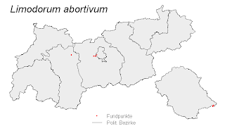
6. simple example for using shapefiles with R, download example data.

# A simple example for drawing an occurrence-map (polygons with species' points) 

# with the R-packages maptools and sp using shapefiles.

library(maptools)

library(sp)



# Note that for each shapefile, you only need to read the .shp component

# the others will be read in at the same time automatically.

# TIRIS.BEZIDX_PL.shp contains the political districts of North-Tyrol

# Limodorum.shp contains points with occurences of the plant species

# Limodorum abortivum.

# Note that my layers use the same geographic coordinate systems (gcs),

# using other data you would need to check if the gcs and

# projection of all layers are the same!  



# set dir to where you downloaded the data:

setwd("E:/R/Data/Maps/Example.1_Data")

Limodorum.shp <- readShapePoints(file.choose())

TIRIS.BEZIDX_PL.shp <- readShapePoly(file.choose())



# examine points:

summary(Limodorum.shp)

attributes(Limodorum.shp@data)



# examine polygons:

summary(TIRIS.BEZIDX_PL.shp)

attributes(TIRIS.BEZIDX_PL.shp@data)



# limits:

# to customize ylim in plot-call

# seems not to work here...

xlim <- TIRIS.BEZIDX_PL.shp@bbox[1, ]

ylim <- TIRIS.BEZIDX_PL.shp@bbox[2, ]     



par(mai = rep(.1, 4))



plot(TIRIS.BEZIDX_PL.shp, col = "grey93", axes = F,

     xlim = xlim, ylim = ylim, bty = "n")

points(Limodorum.shp, pch = 16,

       col = 2, cex = .5)

mtext("Limodorum abortivum", 3, line = -7,

      at = -17000, adj = 0, cex = 2, font = 3)

legend("bottomleft", inset = c(0.4, 0.2),

       legend = c("Fundpunkte", "Polit. Bezirke"),

       bty = "n", pch = c(16,-1),           # bty = "n": no box

       col = c(2, 1), pt.cex = c(.5, 1),

       lty = c(-1, 1))

Created by Pretty R at inside-R.org



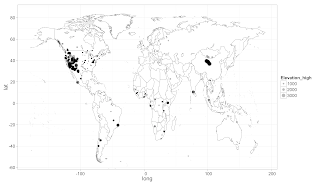
7. Weecology can has new mammal dataset
use the rOpenSci package treebase to search the online phylogeny repository TreeBASE.  Limiting to returning a max of 1 tree (to save time), wecan see that X species are in at least 1 tree on the TreeBASE database.

# setwd("/Mac/R_stuff/Blog_etc/Mammal_Dataset")



# URLs for datasets

comm <- "http://esapubs.org/archive/ecol/E092/201/data/MCDB_communities.csv"

refs <- "http://esapubs.org/archive/ecol/E092/201/data/MCDB_references.csv"

sites <- "http://esapubs.org/archive/ecol/E092/201/data/MCDB_sites.csv"

spp <- "http://esapubs.org/archive/ecol/E092/201/data/MCDB_species.csv"

trap <- "http://esapubs.org/archive/ecol/E092/201/data/MCDB_trapping.csv"



# read them

require(plyr)

datasets <- llply(list(comm, refs, sites, spp, trap), read.csv, .progress='text')

str(datasets[[1]]); head(datasets[[1]]) # cool, worked

llply(datasets, head) # see head of all data.frame's



# Map the communities

require(ggplot2)

require(maps)

sitesdata <- datasets[[3]]

sitesdata <- sitesdata[!sitesdata$Latitude == 'NULL',]

sitesdata$Latitude <- as.numeric(as.character(sitesdata$Latitude))

sitesdata$Longitude <- as.numeric(as.character(sitesdata$Longitude))

sitesdata$Elevation_high <- as.numeric(as.character(sitesdata$Elevation_high))

sitesdata <- sitesdata[sitesdata$Longitude > -140,]

world_map <- map_data("world")

us <- world_map[world_map$region=='USA',]



  # World map

ggplot(world_map, aes(long, lat)) +

  theme_bw(base_size=16) +

  geom_polygon(aes(group = group), colour="grey60", fill = 'white', size = .3) +

  ylim(-55, 85) +

  geom_jitter(data = sitesdata, aes(Longitude, Latitude, size=Elevation_high), alpha=0.3)

ggsave("worldmap.png")



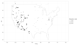
  # US only

ggplot(us, aes(long, lat)) +

  theme_bw(base_size=16) +

  geom_polygon(aes(group = group), colour="grey60", fill = 'white', size = .3) +

  ylim(25, 50) +

  xlim(-130, -60) +

  geom_jitter(data = sitesdata, aes(Longitude, Latitude, size=Elevation_high), alpha=0.3)

ggsave("usmap.png")



# What phylogenies can we get for these species?

install.packages("treebase")

require(treebase); require(RCurl)

datasets[[4]]$gensp <- as.factor(paste(datasets[[4]]$Genus, datasets[[4]]$Species))



trees <- llply(datasets[[4]]$gensp, function(x) search_treebase(paste("\"", x, '\"', sep=''),

          by="taxon", max_trees=1, exact_match=TRUE, curl=getCurlHandle()))

spwithtrees <- data.frame(datasets[[4]]$gensp,

           laply(trees, function(x) if(length(unlist(x)) > 0){1} else{0}))

names(spwithtrees) <- c('species', 'trees')

length(spwithtrees[spwithtrees$trees == 1, 2])

Created by Pretty R at inside-R.org



8. googleVis 0.2.13: new stepped area chart and improved geo charts

you should go to the post to see the nice plots.

9. Spatial Data with R, two videos on how to do


10.  Create maps with maptools R package

library(maptools)

france<-readShapeSpatial("departements.shp",

  proj4string=CRS("+proj=longlat"))

routesidf<-readShapeLines(

  "ile-de-france.shp/roads.shp",

  proj4string=CRS("+proj=longlat")

  )

trainsidf<-readShapeLines(

  "ile-de-france.shp/railways.shp",

  proj4string=CRS("+proj=longlat")

  )

plot(france,xlim=c(2.2,2.4),ylim=c(48.75,48.95),lwd=2)

plot(routesidf[routesidf$type=="secondary",],add=TRUE,lwd=2,col="lightgray")

plot(routesidf[routesidf$type=="primary",],add=TRUE,lwd=2,col="lightgray")

plot(trainsidf[trainsidf$type=="rail",],add=TRUE,lwd=1,col="burlywood3")

points(eglises$lon,eglises$lat,pch=20,col="red")

Created by Pretty R at inside-R.org



11. Producing Google Map Embeds with R Package googleVis

the output plot, http://localhost:21131/custom/googleVis/MapID3bdbc9a1.html

# (1) for producing html code for a Google Map with R-package googleVis do something like:

library(googleVis)

df <- data.frame(Address = c("Innsbruck", "Wattens"),

                 Tip = c("My Location 1", "My Location 2"))

mymap <- gvisMap(df, "Address", "Tip", options = list(showTip = TRUE, mapType = "normal",

                 enableScrollWheel = TRUE))

plot(mymap) # preview



# (2) then just copy-paste the html to your blog or website after customizing for your purpose..

Created by Pretty R at inside-R.org



12. Retrieve GBIF Species Occurrence Data with Function from dismo Package
The dismo package is awesome: with some short lines of code you can read & map species distribution data from GBIF (theglobal biodiversity information facility)

<div style="overflow:auto;">

library(dismo)



# get GBIF data with function:

myrger <- gbif("Myricaria", "germanica", geo = T)



# check:

str(myrger)



# plot occurrences:

library(maptools)

data(wrld_simpl)

plot(wrld_simpl, col = "light yellow", axes = T)

points(myrger$lon, myrger$lat, col = "red", cex = 0.5)

text(-140, -50, "MYRICARIA\nGERMANICA")

Created by Pretty R at inside-R.org



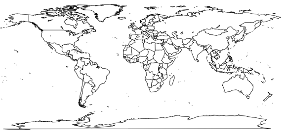
13. The Global Earthquake Desktop
The U.S. Geological Survey (USGS) provides feeds and data catalogs of the latestearthquakes, which can be found here.


The maps package in R is great for producing simple maps of data and coding up ourearthquake map is pretty straightforward.

# load the maps library

library(maps)



# get the earthquake data from the USGS

eq <- read.csv("http://earthquake.usgs.gov/earthquakes/catalogs/eqs7day-M2.5.txt", sep = ",", header = TRUE)



# size the earthquake symbol areas according to magnitude

radius <- 10^sqrt(eq$Mag)



# create a time stamp for the image

date <- date()



# set the path and file name of the image file

png("Path/To/Your/Image/worldeq.png", width = 1920, height = 1200)



# plot the world map, earthquakes, and time stamp

map(database = "world",col = "#999999", bg = "#000000")

symbols(eq$Lon, eq$Lat, bg = "#99ccff", fg = "#3467cd", lwd = 1, circles = radius, inches = 0.175, add = TRUE)

text(140, -80, labels = date, col = "#999999")

dev.off()

Created by Pretty R at inside-R.org



# run R in terminal, and automatically update the plot every day.

R CMD Batch /Path/To/Your/R/Script/worldeq.R

defaults write com.apple.desktop Background '{default = {ImageFilePath = "/Path/To/Your/Image/worldeq.png"; };}'

killall Dock

14. R Spatial Tips

Intro to Handling Spatial Data with R.

Creating a map with R.

Creating a map with R using ggplot2.

R Interface to Google Charts (Gapminder Style).

R Interface to Google Charts (Mapping).

Exporting KML from R to create maps in Google Earth.

Clipping/ extracting a surface to within a polygon. Includes dissolving polygons.

Writing a spatial function: The Location Quotient.

Creating a TreeMap.

Installing rgdal on Mac OS X.

Mapping Great Circles with R (external site).

Mapping Twitter Followers with R (external site).

Using R as a GIS.

Relevant Book Reviews:

- Applied Spatial Data Analysis with R.

-Lattice: Multivariate Data Visualization with R.

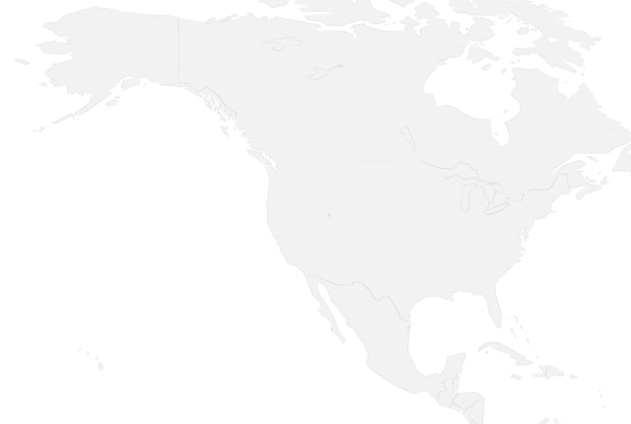
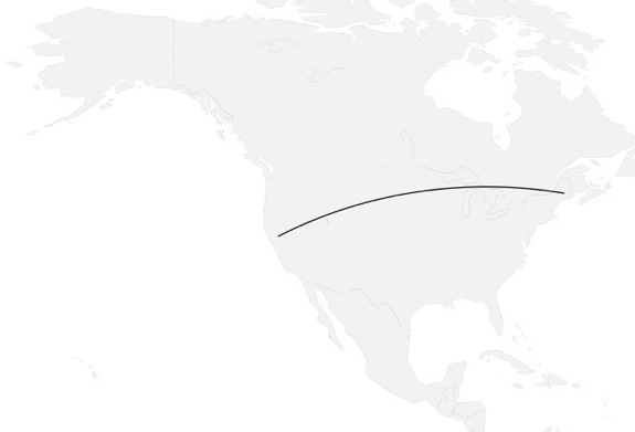
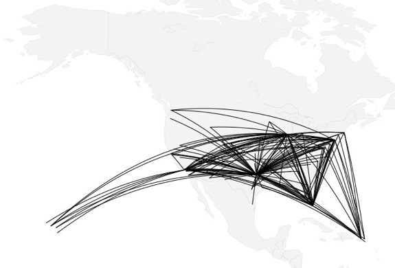
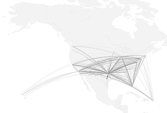
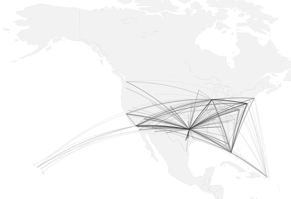
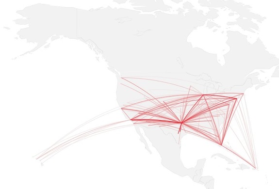
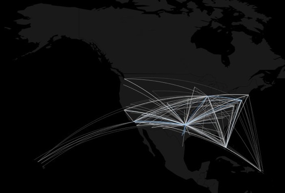
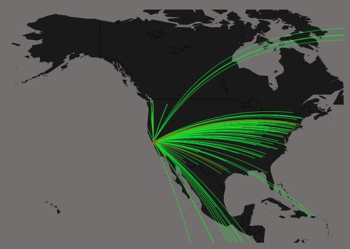
15. how to map connections with great circles

16. migration

https://github.com/aihardin/Academic_Migrations/blob/master/map_students.R

#http://flowingdata.com/2011/05/11/how-to-map-connections-with-great-circles



students <- read.csv('/Users/aaron/projects/graduate_student_migrations/students_2005-2011.txt', header=TRUE, as.is=TRUE)

universities <- read.csv('/Users/aaron/projects/graduate_student_migrations/universities_2005-2011.txt', header=TRUE)



library(maps)

library(geosphere)



checkDateLine <- function(l){

  n<-0

  k<-length(l)

  k<-k-1

  for (j in 1:k){

    n[j] <- l[j+1] - l[j]

  }

  n <- abs(n)

  m<-max(n, rm.na=TRUE)

  ifelse(m > 30, TRUE, FALSE)

}

clean.Inter <- function(p1, p2, n, addStartEnd){

  inter <- gcIntermediate(p1, p2, n=n, addStartEnd=addStartEnd)

  if (checkDateLine(inter[,1])){

    m1 <- midPoint(p1, p2)

    m1[,1] <- (m1[,1]+180)%%360 - 180

    a1 <- antipode(m1)

    l1 <- gcIntermediate(p1, a1, n=n, addStartEnd=addStartEnd)

    l2 <- gcIntermediate(a1, p2, n=n, addStartEnd=addStartEnd)

    l3 <- rbind(l1, l2)

    l3

  }

  else{

    inter

  }

}



#map("world", col="#191919", fill=TRUE, bg="#736F6E", lwd=0.05)





add_lines <- function(){

  pal <- colorRampPalette(c("#00FF00", "#FF0000"))

  colors <- pal(100)



  fsub <- students[order(students$cnt),]

  maxcnt <- max(fsub$cnt)

  for (j in 1:length(fsub$undergrad)) {

    u1 <- universities[universities$uni_id == fsub[j,]$undergrad,]

    u2 <- universities[universities$uni_id == fsub[j,]$grad,]

    p1 <- c(u1[1,]$long, u1[1,]$lat)

    p2 <- c(u2[1,]$long, u2[1,]$lat)

    inter <- clean.Inter(p1,p2,n=100, addStartEnd=TRUE)

    colindex <- round( (fsub[j,]$cnt / maxcnt) *length(colors))

    lines(inter, col=colors[colindex], lwd=0.6)

  }

}



map_usa <- function(){

  xlim <- c(-171.738281, -56.601563)

  ylim <- c(12.039321, 71.856229)

  map("world", col="#191919", fill=TRUE, bg="#736F6E", lwd=0.05, xlim=xlim, ylim=ylim)

  add_lines()

}



map_world <- function(){

  map("world", col="#191919", fill=TRUE, bg="#736F6E", lwd=0.05)

  add_lines()

}

map_usa()

Created by Pretty R at inside-R.org



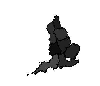
17. Amateur Mapmaking: Getting Started With Shapefiles

01	#Download English Government Office Network Regions (GOR) from:

02	#http://www.sharegeo.ac.uk/handle/10672/50

03	#Unzip and change directory name to something like UK_GORs

04

05	#We definitely need maptools - you may need to download and install this package first

06	library(maptools)

07

08	#Load in the data file (could this be done from the downloaded zip file directly?

09	gor=readShapeSpatial('~/Downloads/UK_GORs/Regions.shp')

10

11	#I can plot the shapefile okay...

12

plot(gor)

02	summary(gor)

03	attributes(gor@data)

04	gor@data$NAME

05	#[1] North East               North West

06	#[3] Greater London Authority West Midlands

07	#[5] Yorkshire and The Humber South West

08	#[7] East Midlands            South East

09	#[9] East of England

10	#9 Levels: East Midlands East of England ... Yorkshire and The Humber

11

12	#download data from http://www.justice.gov.uk/downloads/publications/statistics-and-data/courts-and-sentencing/csq-q3-2011-insolvency-tables.csv

13	insolvency<- read.csv("~/Downloads/csq-q3-2011-insolvency-tables.csv")

14	#Grab a subset of the data, specifically to Q3 2011 and numbers that are aggregated by GOR

15	insolvencygor.2011Q3=subset(insolvency,Time.Period=='2011 Q3' & Geography.Type=='Government office region')

16

17	#tidy the data - you may need to download and install the gdata package first

18	#The subsetting step doesn't remove extraneous original factor levels, so I will.

19	require(gdata)

20	insolvencygor.2011Q3=drop.levels(insolvencygor.2011Q3)

21

22	names(insolvencygor.2011Q3)

23	#[1] "Time.Period"                 "Geography"

24	#[3] "Geography.Type"              "Company.Winding.up.Petition"

25	#[5] "Creditors.Petition"          "Debtors.Petition"

26

27	levels(insolvencygor.2011Q3$Geography)

28	#[1] "East"                     "East Midlands"

29	#[3] "London"                   "North East"

30	#[5] "North West"               "South East"

31	#[7] "South West"               "Wales"

32	#[9] "West Midlands"            "Yorkshire and the Humber"

33	#Note that these names for the GORs don't quite match the ones used in the shapefile, though how they relate one to another is obvious to us...

34

35	#So what next? [That was the original question...!]

36

37	#Here's the answer I came up with...

38	#Convert factors to numeric [ http://stackoverflow.com/questions/4798343/convert-factor-to-integer ]

39	#There's probably a much better formulaic way of doing this/automating this?

40	insolvencygor.2011Q3$Creditors.Petition=as.numeric(levels(insolvencygor.2011Q3$Creditors.Petition))[insolvencygor.2011Q3$Creditors.Petition]

41	insolvencygor.2011Q3$Company.Winding.up.Petition=as.numeric(levels(insolvencygor.2011Q3$Company.Winding.up.Petition))[insolvencygor.2011Q3$Company.Winding.up.Petition]

42	insolvencygor.2011Q3$Debtors.Petition=as.numeric(levels(insolvencygor.2011Q3$Debtors.Petition))[insolvencygor.2011Q3$Debtors.Petition]

43

44	#Tweak the levels so they match exactly (really should do this via a lookup table of some sort?)

45	i2=insolvencygor.2011Q3

46	i2c=c('East of England','East Midlands','Greater London Authority','North East','North West','South East','South West','Wales','West Midlands','Yorkshire and The Humber')

47	i2$Geography=factor(i2$Geography,labels=i2c)

48

49	#Merge the data with the shapefile

50	gor@data=merge(gor@data,i2,by.x='NAME',by.y='Geography')

51

52	#Plot the data using a greyscale

53	plot(gor,col=gray(gor@data$Creditors.Petition/max(gor@data$Creditors.Petition)))

17. retrive data from Global Administrative Areas (GADM) and plot with ggplot2

library(ggplot2)

library(gpclib)

library(plyr) 

library(maptools) 

load(url("http://gadm.org/data/rda/JPN_adm2.RData")) 

 

# restricted licence (see: http://www.cs.man.ac.uk/~toby/alan/software/#Licensing)

gpclibPermit() 

# which variable identifies polygons?

head(as.data.frame(gadm)) 

# looks like ID_2

# convert to a structure ggplot2 can handle...takes a while

japan_map <- fortify(gadm, region = "ID_2") 

# join up the useful names

japan_map <- rename(japan_map, c("id" = "ID_2")) 

japan_map <- join(japan_map,  as.data.frame(gadm)[, c("ID_2", "NAME_1", "NAME_2")]) 

# a subset for speed

qplot(long, lat, data = subset(japan_map, NAME_1 == "Miyagi"), geom = "path", group = group) 

# filled polygons

qplot(long, lat, data = subset(japan_map, NAME_1 == "Miyagi"), geom = "polygon", group = group) 

# everything = SLOW!

qplot(long, lat, data = japan_map, geom = "path", group = group) 

# everything, filled polygons

qplot(long, lat, data = japan_map, geom = "polygon", group = group) 

 

# add points with size defined by populations

ggplot() + geom_path(aes(x=long, y=lat, group=group), data=japan_map) 

+ geom_point(aes(x=long, y=lat, size = population), data=Region) 

 

ggplot(mapping=aes(x=long, y=lat)) + geom_path(aes(group=group), 

data=japan_map) + geom_point(aes(size = population), data=Region)

Created by Pretty R at inside-R.org