We study diverse topics in evolutionary genetics, but focus on the evolution of populations that are distributed through space, and that experience natural selection on many genes. Understanding how species adapt, and how they split into new species, requires knowledge of the effects of spatial subdivision; conversely, spatial patterns can tell us about the strengths of evolutionary processes that are hard to measure directly. Interactions between large numbers of genes are important in species formation, in the response to natural and artificial selection, and in the net effects of selection on the whole genome. The recent development of techniques for assaying large numbers of genetic markers, and indeed complete sequences, make analysis of the interactions amongst large numbers of genes essential.
http://ist.ac.at/research-groups-pages/barton-group/
2013年7月30日星期二
2013年7月29日星期一
Agalma: an automated phylogenomics workflow
1. Agalma: an automated phylogenomics workflow
http://arxiv.org/abs/1307.7313
2. https://bitbucket.org/caseywdunn/agalma
http://arxiv.org/abs/1307.7313
2. https://bitbucket.org/caseywdunn/agalma
2013年7月28日星期日
Inferring Demographic History from a Spectrum of Shared Haplotype Lengths
There has been much recent excitement about the use of genetics to elucidate ancestral history and demography. Whole genome data from humans and other species are revealing complex stories of divergence and admixture that were left undiscovered by previous smaller data sets. A central challenge is to estimate the timing of past admixture and divergence events, for example the time at which Neanderthals exchanged genetic material with humans and the time at which modern humans left Africa. Here, we present a method for using sequence data to jointly estimate the timing and magnitude of past admixture events, along with population divergence times and changes in effective population size. We infer demography from a collection of pairwise sequence alignments by summarizing their length distribution of tracts of identity by state (IBS) and maximizing an analytic composite likelihood derived from a Markovian coalescent approximation. Recent gene flow between populations leaves behind long tracts of identity by descent (IBD), and these tracts give our method power by influencing the distribution of shared IBS tracts. In simulated data, we accurately infer the timing and strength of admixture events, population size changes, and divergence times over a variety of ancient and recent time scales. Using the same technique, we analyze deeply sequenced trio parents from the 1000 Genomes project. The data show evidence of extensive gene flow between Africa and Europe after the time of divergence as well as substructure and gene flow among ancestral hominids. In particular, we infer that recent African-European gene flow and ancient ghost admixture into Europe are both necessary to explain the spectrum of IBS sharing in the trios, rejecting simpler models that contain less population structure.
Identifying differential alternative splicing events from RNA sequencing data
http://www.mimg.ucla.edu/faculty/xing/index.html
Zhao K., Lu ZX., Park JW., Zhou Q., Xing Y. (2013) GLiMMPS: Robust statistical model for regulatory variation of alternative splicing using RNA-Seq data, Genome Biology, 14:R74. [journal] [GLiMMPS software]
Park JW., Tokheim C., Shen S., Xing Y. (2013) Identifying differential alternative splicing events from RNA sequencing data using RNASeq-MATS. Methods in Molecular Biology: Deep Sequencing Data Analysis, Invited Book Chapter,1038:171-179. [book] [PubMed]
driftsel: an R package for detecting signals of natural selection in quantitative traits
http://onlinelibrary.wiley.com/doi/10.1111/1755-0998.12111/full
Approaches and tools to differentiate between natural selection and genetic drift as causes of population differentiation are of frequent demand in evolutionary biology. Based on the approach of Ovaskainen et al. (2011), we have developed an R package (driftsel) that can be used to differentiate between stabilizing selection, diversifying selection and random genetic drift as causes of population differentiation in quantitative traits when neutral marker and quantitative genetic data are available. Apart from illustrating the use of this method and the interpretation of results using simulated data, we apply the package on data from three-spined sticklebacks (Gasterosteus aculeatus) to highlight its virtues. driftsel can also be used to perform usual quantitative genetic analyses in common-garden study designs.
Approaches and tools to differentiate between natural selection and genetic drift as causes of population differentiation are of frequent demand in evolutionary biology. Based on the approach of Ovaskainen et al. (2011), we have developed an R package (driftsel) that can be used to differentiate between stabilizing selection, diversifying selection and random genetic drift as causes of population differentiation in quantitative traits when neutral marker and quantitative genetic data are available. Apart from illustrating the use of this method and the interpretation of results using simulated data, we apply the package on data from three-spined sticklebacks (Gasterosteus aculeatus) to highlight its virtues. driftsel can also be used to perform usual quantitative genetic analyses in common-garden study designs.
2013年7月18日星期四
Pipit: visualizing functional impacts of structural variations
Summary: Pipit is a gene-centric interactive visualization tool designed to study structural genomic variations. Through focusing on individual genes as the functional unit, researchers are able to study and generate hypotheses on the biological impact of different structural variations, for instance, the deletion of dosage-sensitive genes or the formation of fusion genes. Pipit is a cross-platform Java application that visualizes structural variation data from Genome Variation Format files.
Availability: Executables, source code, sample data, documentation and screencast are available at https://bitbucket.org/biovizleuven/pipit.
Inferring Demography from Runs of Homozygosity in Whole Genome Sequence, with Correction for Sequence Errors
Whole genome sequence is potentially the richest source of genetic data for inferring ancestral demography. However, full sequence also presents significant challenges to fully utilize such large data sets and to ensure that sequencing errors do not introduce bias into the inferred demography. Using whole genome sequence data from two Holstein cattle, we demonstrate a new method to correct for bias caused by hidden errors and then infer stepwise changes in ancestral demography up to present. There was a strong upward bias in estimates of recent effective population size (Ne) if the correction method was not applied to the data, both for our method and the Li and Durbin (2011) PSMC method. To infer demography, we use an analytical predictor of multiloci linkage disequilibrium (LD) based on a simple coalescent model that allows for changes in Ne. The LD statistic summarises the distribution of runs of homozygosity for any given demography. We infer a best fit demography as one that predicts a match with the observed distribution of runs of homozygosity in the corrected sequence data. We use multiloci LD because it potentially holds more information about ancestral demography than pairwise LD. The inferred demography indicates a strong reduction in the Ne around 170,000 years ago, possibly related to the divergence of African and European Bos taurus cattle. This is followed by a further reduction coinciding with the period of cattle domestication, with Ne of between 3,500 and 6,000. The most recent reduction of Ne to approximately 100 in the Holstein breed agrees well with estimates from pedigrees. Our approach can be applied to whole genome sequence from any diploid species and can be scaled up to use sequence from multiple individuals.
Our inference method can be applied to any
outbred diploid species for one or multiple individuals without the need to phase the data into
haplotypes.
http://mbe.oxfordjournals.org/content/early/2013/07/10/molbev.mst125.abstract
Our inference method can be applied to any
outbred diploid species for one or multiple individuals without the need to phase the data into
haplotypes.
http://mbe.oxfordjournals.org/content/early/2013/07/10/molbev.mst125.abstract
2013年7月15日星期一
Java utilities for NGS - Jvarkit
https://github.com/lindenb/jvarkit#vcfgeneontology
http://plindenbaum.blogspot.ca/
Example:
Example:
http://plindenbaum.blogspot.ca/
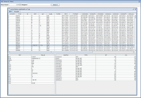
VcfViewGui
VcfViewGui : a Simple java-Swing-based VCF viewer.VCFGeneOntology
vcfgo reads a VCF annotated with VEP or SNPEFF, loads the data from GeneOntology andGOA and adds a new field in the INFO column for the GO terms for each position.Example:
$ java -jar dist/vcfgo.jar I="https://raw.github.com/arq5x/gemini/master/test/tes.snpeff.vcf" |\
    grep -v -E '^##' | head -n 3

#CHROM  POS ID  REF ALT QUAL    FILTER  INFO    FORMAT  1094PC0005  1094PC0009  1094PC0012  1094PC0013
chr1    30860   .   G   C   33.46   .   AC=2;AF=0.053;AN=38;BaseQRankSum=2.327;DP=49;Dels=0.00;EFF=DOWNSTREAM(MODIFIER||||85|FAM138A|protein_coding|CODING|ENST00000417324|),DOWNSTREAM(MODIFIER|||||FAM138A|processed_transcript|CODING|ENST00000461467|),DOWNSTREAM(MODIFIER|||||MIR1302-10|miRNA|NON_CODING|ENST00000408384|),INTRON(MODIFIER|||||MIR1302-10|antisense|NON_CODING|ENST00000469289|),INTRON(MODIFIER|||||MIR1302-10|antisense|NON_CODING|ENST00000473358|),UPSTREAM(MODIFIER|||||WASH7P|unprocessed_pseudogene|NON_CODING|ENST00000423562|),UPSTREAM(MODIFIER|||||WASH7P|unprocessed_pseudogene|NON_CODING|ENST00000430492|),UPSTREAM(MODIFIER|||||WASH7P|unprocessed_pseudogene|NON_CODING|ENST00000438504|),UPSTREAM(MODIFIER|||||WASH7P|unprocessed_pseudogene|NON_CODING|ENST00000488147|),UPSTREAM(MODIFIER|||||WASH7P|unprocessed_pseudogene|NON_CODING|ENST00000538476|);FS=3.128;HRun=0;HaplotypeScore=0.6718;InbreedingCoeff=0.1005;MQ=36.55;MQ0=0;MQRankSum=0.217;QD=16.73;ReadPosRankSum=2.017 GT:AD:DP:GQ:PL  0/0:7,0:7:15.04:0,15,177    0/0:2,0:2:3.01:0,3,39   0/0:6,0:6:12.02:0,12,143    0/0:4,0:4:9.03:0,9,119
chr1    69270   .   A   G   2694.18 .   AC=40;AF=1.000;AN=40;DP=83;Dels=0.00;EFF=SYNONYMOUS_CODING(LOW|SILENT|tcA/tcG|S60|305|OR4F5|protein_coding|CODING|ENST00000335137|exon_1_69091_70008);FS=0.000;GOA=OR4F5|GO:0004984&GO:0005886&GO:0004930&GO:0016021;HRun=0;HaplotypeScore=0.0000;InbreedingCoeff=-0.0598;MQ=31.06;MQ0=0;QD=32.86   GT:AD:DP:GQ:PL  ./. ./. 1/1:0,3:3:9.03:106,9,0  1/1:0,6:6:18.05:203,18,0
VCFFilterGeneOntology
vcffiltergo reads a VCF annotated with VEP or SNPEFF, loads the data from GeneOntologyand GOA and adds a filter in the FILTER column if a gene at the current genomic location is a descendant of a given GO term.Example:
$  java -jar dist/vcffiltergo.jar I="https://raw.github.com/arq5x/gemini/master/test/test1.snpeff.vcf"  \
    CHILD_OF=GO:0005886 FILTER=MEMBRANE  |\
    grep -v "^##"   | head -n 3

#CHROM  POS ID  REF ALT QUAL    FILTER  INFO    FORMAT  1094PC0005  1094PC0009  1094PC0012  1094PC0013
chr1    30860   .   G   C   33.46   PASS    AC=2;AF=0.053;AN=38;BaseQRankSum=2.327;DP=49;Dels=0.00;EFF=DOWNSTREAM(MODIFIER||||85|FAM138A|protein_coding|CODING|ENST00000417324|),DOWNSTREAM(MODIFIER|||||FAM138A|processed_transcript|CODING|ENST00000461467|),DOWNSTREAM(MODIFIER|||||MIR1302-10|miRNA|NON_CODING|ENST00000408384|),INTRON(MODIFIER|||||MIR1302-10|antisense|NON_CODING|ENST00000469289|),INTRON(MODIFIER|||||MIR1302-10|antisense|NON_CODING|ENST00000473358|),UPSTREAM(MODIFIER|||||WASH7P|unprocessed_pseudogene|NON_CODING|ENST00000423562|),UPSTREAM(MODIFIER|||||WASH7P|unprocessed_pseudogene|NON_CODING|ENST00000430492|),UPSTREAM(MODIFIER|||||WASH7P|unprocessed_pseudogene|NON_CODING|ENST00000438504|),UPSTREAM(MODIFIER|||||WASH7P|unprocessed_pseudogene|NON_CODING|ENST00000488147|),UPSTREAM(MODIFIER|||||WASH7P|unprocessed_pseudogene|NON_CODING|ENST00000538476|);FS=3.128;HRun=0;HaplotypeScore=0.6718;InbreedingCoeff=0.1005;MQ=36.55;MQ0=0;MQRankSum=0.217;QD=16.73;ReadPosRankSum=2.017 GT:AD:DP:GQ:PL  0/0:7,0:7:15.04:0,15,177    0/0:2,0:2:3.01:0,3,39   0/0:6,0:6:12.02:0,12,143    0/0:4,0:4:9.03:0,9,119
chr1    69270   .   A   G   2694.18 MEMBRANE    AC=40;AF=1.000;AN=40;DP=83;Dels=0.00;EFF=SYNONYMOUS_CODING(LOW|SILENT|tcA/tcG|S60|305|OR4F5|protein_coding|CODING|ENST00000335137|exon_1_69091_70008);FS=0.000;HRun=0;HaplotypeScore=0.0000;InbreedingCoeff=-0.0598;MQ=31.06;MQ0=0;QD=32.86 GT:AD:DP:GQ:PL  ./. ./. 1/1:0,3:3:9.03:106,9,0  1/1:0,6:6:18.05:203,18,0
2013年7月12日星期五
choose colors for your plots
1. The HTML 4.01 specification[9] defines sixteen named colors, as follows (names are defined in this context to be case-insensitive):
http://en.wikipedia.org/wiki/Web_colors
2. using colors in R
http://en.wikipedia.org/wiki/Web_colors
| Color | Name | Hex (RGB) | Red (RGB) | Green (RGB) | Blue (RGB) | Hue (HSL/HSV) | Satur (HSL) | Light (HSL) | Satur (HSV) | Value (HSV) | CGA number (name); alias |
|---|---|---|---|---|---|---|---|---|---|---|---|
| White | #FFFFFF | 100% | 100% | 100% | 0° | 0% | 100% | 0% | 100% | 15 (white) | |
| Silver | #C0C0C0 | 75% | 75% | 75% | 0° | 0% | 75% | 0% | 75% | 7 (light gray) | |
| Gray | #808080 | 50% | 50% | 50% | 0° | 0% | 50% | 0% | 50% | 8 (dark gray) | |
| Black | #000000 | 0% | 0% | 0% | 0° | 0% | 0% | 0% | 0% | 0 (black) | |
| Red | #FF0000 | 100% | 0% | 0% | 0° | 100% | 50% | 100% | 100% | 12 (high red) | |
| Maroon | #800000 | 50% | 0% | 0% | 0° | 100% | 25% | 100% | 50% | 4 (low red) | |
| Yellow | #FFFF00 | 100% | 100% | 0% | 60° | 100% | 50% | 100% | 100% | 14 (yellow) | |
| Olive | #808000 | 50% | 50% | 0% | 60° | 100% | 25% | 100% | 50% | 6 (brown) | |
| Lime | #00FF00 | 0% | 100% | 0% | 120° | 100% | 50% | 100% | 100% | 10 (high green); green | |
| Green | #008000 | 0% | 50% | 0% | 120° | 100% | 25% | 100% | 50% | 2 (low green) | |
| Aqua | #00FFFF | 0% | 100% | 100% | 180° | 100% | 50% | 100% | 100% | 11 (high cyan); cyan | |
| Teal | #008080 | 0% | 50% | 50% | 180° | 100% | 25% | 100% | 50% | 3 (low cyan) | |
| Blue | #0000FF | 0% | 0% | 100% | 240° | 100% | 50% | 100% | 100% | 9 (high blue) | |
| Navy | #000080 | 0% | 0% | 50% | 240° | 100% | 25% | 100% | 50% | 1 (low blue) | |
| Fuchsia | #FF00FF | 100% | 0% | 100% | 300° | 100% | 50% | 100% | 100% | 13 (high magenta); magenta | |
| Purple | #800080 | 50% | 0% | 50% | 300° | 100% | 25% | 100% | 50% | 5 (low magenta) |
http://research.stowers-institute.org/efg/Report/UsingColorInR.pdf
| interior | font | HTML | bgcolor= | Red< | Green | Blue | Color |
| Black | [Color 1] | #000000 | #000000 | 0 | 0 | 0 | [Black] |
| White | [Color 2] | #FFFFFF | #FFFFFF | 255 | 255 | 255 | [White] |
| Red | [Color 3] | #FF0000 | #FF0000 | 255 | 0 | 0 | [Red] |
| Green | [Color 4] | #00FF00 | #00FF00 | 0 | 255 | 0 | [Green] |
| Blue | [Color 5] | #0000FF | #0000FF | 0 | 0 | 255 | [Blue] |
| Yellow | [Color 6] | #FFFF00 | #FFFF00 | 255 | 255 | 0 | [Yellow] |
| Magenta | [Color 7] | #FF00FF | #FF00FF | 255 | 0 | 255 | [Magenta] |
| Cyan | [Color 8] | #00FFFF | #00FFFF | 0 | 255 | 255 | [Cyan] |
| [Color 9] | [Color 9] | #800000 | #800000 | 128 | 0 | 0 | [Color 9] |
| [Color 10] | [Color 10] | #008000 | #008000 | 0 | 128 | 0 | [Color 10] |
| [Color 11] | [Color 11] | #000080 | #000080 | 0 | 0 | 128 | [Color 11] |
| [Color 12] | [Color 12] | #808000 | #808000 | 128 | 128 | 0 | [Color 12] |
| [Color 13] | [Color 13] | #800080 | #800080 | 128 | 0 | 128 | [Color 13] |
| [Color 14] | [Color 14] | #008080 | #008080 | 0 | 128 | 128 | [Color 14] |
| [Color 15] | [Color 15] | #C0C0C0 | #C0C0C0 | 192 | 192 | 192 | [Color 15] |
| [Color 16] | [Color 16] | #808080 | #808080 | 128 | 128 | 128 | [Color 16] |
| [Color 17] | [Color 17] | #9999FF | #9999FF | 153 | 153 | 255 | [Color 17] |
| [Color 18] | [Color 18] | #993366 | #993366 | 153 | 51 | 102 | [Color 18] |
| [Color 19] | [Color 19] | #FFFFCC | #FFFFCC | 255 | 255 | 204 | [Color 19] |
| [Color 20] | [Color 20] | #CCFFFF | #CCFFFF | 204 | 255 | 255 | [Color 20] |
| [Color 21] | [Color 21] | #660066 | #660066 | 102 | 0 | 102 | [Color 21] |
| [Color 22] | [Color 22] | #FF8080 | #FF8080 | 255 | 128 | 128 | [Color 22] |
| [Color 23] | [Color 23] | #0066CC | #0066CC | 0 | 102 | 204 | [Color 23] |
| [Color 24] | [Color 24] | #CCCCFF | #CCCCFF | 204 | 204 | 255 | [Color 24] |
| [Color 25] | [Color 25] | #000080 | #000080 | 0 | 0 | 128 | [Color 25] |
| [Color 26] | [Color 26] | #FF00FF | #FF00FF | 255 | 0 | 255 | [Color 26] |
| [Color 27] | [Color 27] | #FFFF00 | #FFFF00 | 255 | 255 | 0 | [Color 27] |
| [Color 28] | [Color 28] | #00FFFF | #00FFFF | 0 | 255 | 255 | [Color 28] |
| [Color 29] | [Color 29] | #800080 | #800080 | 128 | 0 | 128 | [Color 29] |
| [Color 30] | [Color 30] | #800000 | #800000 | 128 | 0 | 0 | [Color 30] |
| [Color 31] | [Color 31] | #008080 | #008080 | 0 | 128 | 128 | [Color 31] |
| [Color 32] | [Color 32] | #0000FF | #0000FF | 0 | 0 | 255 | [Color 32] |
| [Color 33] | [Color 33] | #00CCFF | #00CCFF | 0 | 204 | 255 | [Color 33] |
| [Color 34] | [Color 34] | #CCFFFF | #CCFFFF | 204 | 255 | 255 | [Color 34] |
| [Color 35] | [Color 35] | #CCFFCC | #CCFFCC | 204 | 255 | 204 | [Color 35] |
| [Color 36] | [Color 36] | #FFFF99 | #FFFF99 | 255 | 255 | 153 | [Color 36] |
| [Color 37] | [Color 37] | #99CCFF | #99CCFF | 153 | 204 | 255 | [Color 37] |
| [Color 38] | [Color 38] | #FF99CC | #FF99CC | 255 | 153 | 204 | [Color 38] |
| [Color 39] | [Color 39] | #CC99FF | #CC99FF | 204 | 153 | 255 | [Color 39] |
| [Color 40] | [Color 40] | #FFCC99 | #FFCC99 | 255 | 204 | 153 | [Color 40] |
| [Color 41] | [Color 41] | #3366FF | #3366FF | 51 | 102 | 255 | [Color 41] |
| [Color 42] | [Color 42] | #33CCCC | #33CCCC | 51 | 204 | 204 | [Color 42] |
| [Color 43] | [Color 43] | #99CC00 | #99CC00 | 153 | 204 | 0 | [Color 43] |
| [Color 44] | [Color 44] | #FFCC00 | #FFCC00 | 255 | 204 | 0 | [Color 44] |
| [Color 45] | [Color 45] | #FF9900 | #FF9900 | 255 | 153 | 0 | [Color 45] |
| [Color 46] | [Color 46] | #FF6600 | #FF6600 | 255 | 102 | 0 | [Color 46] |
| [Color 47] | [Color 47] | #666699 | #666699 | 102 | 102 | 153 | [Color 47] |
| [Color 48] | [Color 48] | #969696 | #969696 | 150 | 150 | 150 | [Color 48] |
| [Color 49] | [Color 49] | #003366 | #003366 | 0 | 51 | 102 | [Color 49] |
| [Color 50] | [Color 50] | #339966 | #339966 | 51 | 153 | 102 | [Color 50] |
| [Color 51] | [Color 51] | #003300 | #003300 | 0 | 51 | 0 | [Color 51] |
| [Color 52] | [Color 52] | #333300 | #333300 | 51 | 51 | 0 | [Color 52] |
| [Color 53] | [Color 53] | #993300 | #993300 | 153 | 51 | 0 | [Color 53] |
| [Color 54] | [Color 54] | #993366 | #993366 | 153 | 51 | 102 | [Color 54] |
| [Color 55] | [Color 55] | #333399 | #333399 | 51 | 51 | 153 | [Color 55] |
| [Color 56] | [Color 56] | #333333 | #333333 | 51 | 51 | 51 | [Color 56] |
| Excel only recognizes names for Color 1 through 8 (Black, White, Red, Green, Blue, Yellow, Magenta, and Cyan). The colors 1-16 are widely understood color names from the VGA color palette. Of the 56 colors only 40 colors appear on the palette. The 40 colors names indicated on the Excel color palette (see below) are for descriptive purposes only. | |||||||
订阅:
博文 (Atom)