2012年8月27日星期一
2012年8月17日星期五
3 blogs on statistics and R
1. r-bloggers
http://www.r-bloggers.com/
2. rplanet
http://planetr.stderr.org/
3. statsblogs
http://www.statsblogs.com/
http://www.r-bloggers.com/
2. rplanet
http://planetr.stderr.org/
3. statsblogs
http://www.statsblogs.com/
2012年7月18日星期三
2012年6月13日星期三
2012年6月8日星期五
Shared spatial effects on quantitative genetic parameters
http://onlinelibrary.wiley.com/doi/10.1111/j.1558-5646.2012.01620.x/full
Linear mixed-effects models (LMMs) were conducted in ASReml3 (VSN International, Hemel Hempsted, UK; Gilmore et al. 2009). We used two techniques to incorporate spatial information into the models . First , we fitted average lifetime spatial coordinates as ordered row and column effects , fitted as additional random effects , with a covariance structure that assumed a first-order separable autoregressive process to account for spatial dependence (AR1 × AR1, Gilmour et al. 1997). Second, we incorporated information on home range overlap between individuals into the animal model by fitting a vector of shared home range effects as an additional random effect, with the corresponding covariance matrix 
, where S is the home range overlap matrix (the “S matrix”). For full details of how we incorporated spatial information into linear mixed models, please see File 2 in supporting information.

take care of the heteroscedasticity of erros in your study
http://www.springerlink.com/content/7111wxg10j657q04/
2012年4月11日星期三
2012年3月3日星期六
resources of Bayesian statistics
The following list of resources from my friend, Jin-Long.
Bayesian Inferences Lectures by P. Lam
Review Course: Markov Chains and Monte Carlo Methods
Bayesian Methods
MachineLearning
Bayesian Networks and Graphical Models
Doing Bayesian Data Analysis
Stat 295 Bayesian Inferences
Bayesian Analysis for the Social Sciences
2012年2月21日星期二
2012年2月14日星期二
Evolutionary Quantitative Genetics - course material
There are course materials open sourced by the author, Bruce Walsh.
Notes and powerpoint slides are posted as pdf files. Chapters are draft version from our online site for the second volume, which contains a lot more additional material
Monday, 30 Jan. Basic statistics
- Lecture 1: Basic Statistical tools
- Lecture 2: Matrix algebra
- Notes
- Slides
- R notes: Distributions in R --- Matrix calculations in R
- Lecture 3: Linear models
- Notes: See Lecture 2
- Slides
Tuesday, 31 Jan: Basic Genetics
- Lecture 4: Introduction to Genetics
- Lecture 5: Introduction to Population Genetics
- Notes: See Lecture 3
- Slides
- Lecture 6: Introduction to Quantitative Genetics
- Notes: See Lecture 3
- Slides
- excel file for calculation average effects, variances from genotypes
Wes , 1 Feb: Resemblance between relatives
Thursday 2 Feb: Mixed models estimates of genetic parameters
- Lecture 9: Random effects and mixed models
- Lecture 10: Mixed model estimation of genetic variances
- Notes: see Lecture 5
- Slides
- Class exercise
- Additional reading: Chapter 17
- Lecture 11: Maternal effects
- Slides
- Additional reading: Chapter 21
Friday 3 Feb: Inbreeding, QTL mapping
Monday, 6 Feb: Tests of Selection
Tuesday, 7 Feb.: Univariate Selection Response
- Lecture 20: Detecting selection using molecular markers II
- Lecture 21: Short term selection response in the mean
- Notes
- Slides
- Additional reading: Chapter 11
- Lecture 22: Short term response in the variance
- Notes
- Slides
- Additional reading: Chapter 22
- Lecture 23: Long-term response
- Slides
- Additional reading: Chapter 23 -- Chapter 24
Wed, 8 Feb: Estimating the fitness of traits
Thursday, 9 Feb: Multivariate response
Friday, 10 Feb: Miscellaneous Advanced topics
- Lecture 30: Associate effects models, kin/group selection, inclusive fitness
- Lecture 31: G x E
- Notes
- Slides
- Additional reading: Chapter 39
- Lecture 32: eQTLs and pathway analysis
- Lecture 33: directed graphs
- Lecture 34: The Infinitesimal model
- Slides
- Additional reading: Chapter 22
2012年2月9日星期四
所有模型都是错的,不过有些挺有用。
As George Box noted: "All models are wrong, some are useful."75
Box, G. E. P. in Robustness in Statistics (eds Launer, R. L. & Wilkinson, G. N.) (Academic Press, New York, 1979).
Box, G. E. P. in Robustness in Statistics (eds Launer, R. L. & Wilkinson, G. N.) (Academic Press, New York, 1979).
2012年1月6日星期五
科学民主在中国 - science, democracy, Communism, economy and others in Chineses books
(1)Chinese words referred in Chinese books
我通过 google 的查询系统,查询了民主(democracy)、科学(science)、共产(Communism)、经济(economy)和其它几个词汇在中午书籍中的引用次数。我不想多解释什么,感兴趣可以看看。
(2)the same sets of words (in English) referred in English books
下面一张是世界范围内,英文书籍上述几种词汇的应用频次。
我通过 google 的查询系统,查询了民主(democracy)、科学(science)、共产(Communism)、经济(economy)和其它几个词汇在中午书籍中的引用次数。我不想多解释什么,感兴趣可以看看。
(2)the same sets of words (in English) referred in English books
下面一张是世界范围内,英文书籍上述几种词汇的应用频次。
2011年12月23日星期五
Markov Chain - interesting and attractive
http://freakonometrics.blog.free.fr/index.php?post/2011/12/20/Basic-on-Markov-Chain-%28for-parents%29
2011年10月27日星期四
正态检验的用途 - 似乎不大 - 要小心
1. Normality tests don't do what most think they do. Shapiro's test, Anderson Darling, and others are null hypothesis tests AGAINST the the assumption of normality. These should not be used to determine whether to use normal theory statistical procedures. In fact they are of virtually no value to the data analyst. Under what conditions are we interested in rejecting the null hypothesis that the data are normally distributed? I have never come across a situation where a normal test is the right thing to do. When the sample size is small, even big departures from normality are not detected, and when your sample size is large, even the smallest deviation from normality will lead to a rejected null.
http://stackoverflow.com/questions/7781798/seeing-if-data-is-normally-distributed-in-r/
2. I, personally, have never come across a situation where a normal test is the right thing to do. The problem is that when the sample size is small, even big departures from normality are not detected, and when your sample size is large, even the smallest deviation from normality will lead to a rejected null.
http://blog.fellstat.com/
2011年10月13日星期四
some sentences on correlation
Correlation measures are among the most basic tools in statistical data analysis and machine learning.
They are applied to pairs of observations to measure to which extent the two observations
comply with a certain model. The most prominent representative is surely Pearson’s product
moment coefficient [1, 13], often nonchalantly called correlation coefficient for short. Pearson’s
product moment coefficient can be applied to numerical data and assumes a linear relationship as
the underlying model; therefore, it can be used to detect linear relationships, but no non-linear
ones.
Rank correlation measures [7, 10, 12] are intended to measure to which extent a monotonic
function is able to model the inherent relationship between the two observables. They neither
assume a specific parametric model nor specific distributions of the observables. They can be
applied to ordinal data and, if some ordering relation is given, to numerical data too. Therefore,
rank correlation measures are ideally suited for detecting monotonic relationships, in particular, if
more specific information about the data is not available. The two most common approaches are
Spearman’s rank correlation coefficient (short Spearman’s rho) [14, 15] and Kendall’s tau (rank
correlation coefficient) [2, 9, 10]. Another simple rank correlation measure is the gamma rank
correlation measure according to Goodman and Kruskal [7].
The rank correlation measures cited above are designed for ordinal data. However, as argued in
[5], they are not ideally suited for measuring rank correlation for numerical data that are perturbed
by noise. Consequently, [5] introduces a family of robust rank correlation measures. The idea
is to replace the classical ordering of real numbers used in Goodman’s and Kruskal’s gamma [7]
by some fuzzy ordering [8, 3, 4] with smooth transitions — thereby ensuring that the correlation
measure is continuous with respect to the data.
cited from "RoCoCo-An R Package Implementing a Robust Rank Correlation Coefficient and a Corresponding Test".
2011年8月19日星期五
Logistic random effects regression models: a comparison of statistical packages for binary and ordinal outcomes
different statistical packages were compared on logistic random effects regression models.
Abstract: Background: Logistic random effects models are a popular tool to analyze multilevel also called hierarchical data with a binary or ordinal outcome. Here, we aim to compare different statistical software implementations of these models.
Methods: We used individual patient data from 8509 patients in 231 centers with moderate and severe Traumatic Brain Injury (TBI) enrolled in eight Randomized Controlled Trials (RCTs) and three observational studies. We fitted logistic random effects regression models with the 5-point Glasgow Outcome Scale (GOS) as outcome, both dichotomized as well as ordinal, with center and/or trial as random effects, and as covariates age, motor score, pupil reactivity or trial. We then compared the implementations of frequentist and Bayesian methods to estimate the fixed and random effects. Frequentist approaches included R (lme4), Stata (GLLAMM), SAS (GLIMMIX and NLMIXED), MLwiN (p[R]IGLS) and MIXOR, Bayesian approaches included WinBUGS, MLwiN (MCMC), R package MCMCglmm and SAS experimental procedure MCMC. Three data sets (the full data set and two sub-datasets) were analysed using basically two logistic random effects models with either one random effect for the center or two random effects for center and trial. For the ordinal outcome in the full data set also a proportional odds model with a random center effect was fitted.
Results: The packages gave similar parameter estimates for both the fixed and random effects and for the binary (and ordinal) models for the main study and when based on a relatively large number of level-1 (patient level) data compared to the number of level-2 (hospital level) data. However, when based on relatively sparse data set, i.e. when the numbers of level-1 and level-2 data units were about the same, the frequentist and Bayesian approaches showed somewhat different results. The software implementations differ considerably in flexibility, computation time, and usability. There are also differences in the availability of additional tools for model evaluation, such as diagnostic plots. The experimental SAS (version 9.2) procedure MCMC appeared to be inefficient.
Conclusions: On relatively large data sets, the different software implementations of logistic random effects regression models produced similar results. Thus, for a large data set there seems to be no explicit preference (of course if there is no preference from a philosophical point of view) for either a frequentist or Bayesian approach (if based on vague priors). The choice for a particular implementation may largely depend on the desired flexibility, and the usability of the package. For small data sets the random effects variances are difficult to estimate. In the frequentist approaches the MLE of this variance was often estimated zero with a standard error that is either zero or could not be determined, while for Bayesian methods the estimates could depend on the chosen "noninformative" prior of the variance parameter. The starting value for the variance parameter may be also critical for the convergence of the Markov chain.
2011年7月7日星期四
understanding correlations by two variables' case
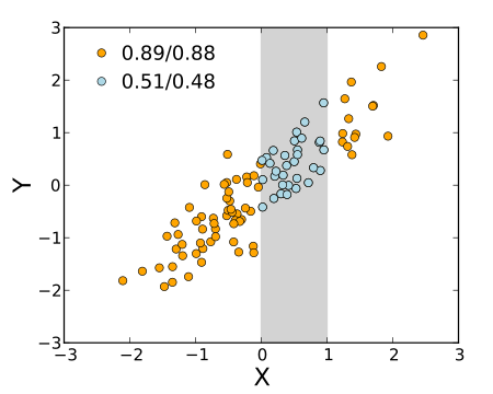
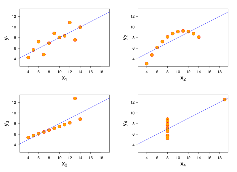
In wiki, there is a really nice introduction to correlation. Here I just grab some nice figures here.
http://en.wikipedia.org/wiki/Correlation_and_dependence
1.
2.
3.
http://en.wikipedia.org/wiki/Correlation_and_dependence
1.
2.
3.
2011年6月17日星期五
订阅:
评论 (Atom)


